E-patterns of age-structured animals for the 21st century
Table of Contents
B) Comparison of Fig. 3 in Heppell et al. (2000) with proposed correction in Mollet and Cailliet (2003, pdf)
C) Fig.3 in Mollet (2005, not published, download pdf with title "Elasticity patterns for sharks, turtles, mammals, and birds: the importance of age at first reproduction, mean age of reproducing females, and survival in the discounted fertilities of the Leslie matrix"). I used 4 hypothetical species with α = 1, 2, 5, and 15 yr to clearly demonstrate that survival in the discounted fertilities needs to be included when calculating the E-pattern
D) Fig.1 in Mollet (2005, not published)
E) What if Sa and m are age-dependent? To be added, covered in Table 3 of Mollet (2005, not published)
F) Fig. 4 in Mollet (2005, not published). Triangle elasticity patterns of elasmobranchs, turtles, mammals, and birds
G) Fig. 1 in Mollet (2004, not published, download pdf). Comment paper on Oli and Dobson (2003) with title: "Elasticity Patterns for Mammals: Age at First Reproduction and Mean Age of Reproducing Females are the Determining Parameters".
H) On the importance of using actual fertility rather than annualized fertility in the calculation of the E-pattern
I) Refutation of major comments by reviewers. Actually covered in Mollet (2005, not published) because I was prepared for everything from the earlier comments on the manuscript submitted to Am Scientist (Mollet, 2004, not published).
A)
Introduction: Why current theory is wrong
Current theory on elasticities (E) of age-structured animals when expressed as an E-pattern using the elasticities of fertility, juvenile survival, and adult survival and graphed in an E-triangle claims that:
1) The E-pattern of a species using a pre-breeding Leslie matrix is different from that using a post-breeding Leslie matrix although the E-matrices are the same.
2) The E-patterns derived from the Leslie matrix (post- or pre-breeding census) are also different from that using a Life History Table (LHT) because the sums of the elasticities are different (1.0 if using a Leslie matrix, 1 + E(m) for LHT). Please note that the Leslie matrices (post- or pre-breeding census) were derived based on the vital rates that were used to construct the LHT.
3) It is acceptable to mix lower- and upper-level parameter when calculating the E-pattern for the Leslie matrix, namely discounted fertility (F, an upper-level parameter) and juvenile survival (Sj) and adult survival (Sa), both lower-level parameters) and use them as the "coordinates" in the E-triangle.
4) We cannot deal with alpha < 1 yr species when using a pre-breeding Leslie matrix.
All these problems are easily fixed if we include the survival rate in the discounted fertilities when calculating the E-pattern for the Leslie matrix (post- or pre-breeding). Now the E-patterns of the Leslie matrix (post-breeding or pre-breeding) are the same and also agree with that of the LHT. Now both post- and pre-breeding E-patterns from the corresponding Leslie matrices and the E-pattern from the LHT only deal with lower-level elasticities (the ones of interest), namely fertility m, juvenile survival Sj, and adult survival Sa. Species with alpha (α) < 1 yr can be dealt with easily in the pre-breeding census.
I have tried to get this published in one comment manuscript on Oli and Dobson (2003) (download pdf) and one 'from scratch' manuscript as a follow-up (download pdf) to Mollet and Cailliet (2003, pdf). Apparently anonymous reviewers and scientific editors require more forceful language. The above items A) - D) make no sense whatsoever. They need to be corrected and are indeed easily corrected if the survival discount in the discounted fertilities is taken into account. I am not going to try a third time to get this published in any scientific journal and "publish" it here. Hopefully it will get accepted and used by the end of 21 century. At least part of it was covered in an Appendix in Mollet and Cailliet (2003, pdf)
Therefore, below I substantiate that the current theory (items 1-4) makes no sense and leads to erroneous conclusions in many cases, in particular for species with age at first reproduction alpha (α) = 1 and 2 yr. I am using Heppell et al. (2000) as an example first. Then I will use several figures from Mollet (2005, unpublished, pdf). I then will deal with Oli and Dobson (2003), who were dealing with mostly alpha (α) = 1 and 2 yr species and therefore most of their elasticities are very much biased and their conclusions are wrong. Finally, I will refute the comments made by the reviewers regarding Mollet (2005, unpublished, pdf).
The "correct" E-patterns are easily calculated using the formulas given in Mollet and Cailliet (2003, Appendix 1b using GP = 0, pdf) and everything is beginning to make sense. For this we only need alpha (α) & Abar (Ā) , where Ā is easily calculated from the defining equation of Ā or using the equation Ā = <w,v> when choosing w1 = 1 and v1 = 1. I also present a new explicit formula for Ā (valid if m and Sa are constant). With this expression for Ā, the elasticity ratio E3/E2 can be calculated explicitly from the vital rates and λ and it can be shown on theoretical grounds that elasmobranchs all have similar E-patterns and that the E3/E2 ratio is always < 1 (the elasticity of juvenile survival is always larger than the elasticity of adult survival) without further considerations because ω/α is < 3 for most elasmobranchs. As a simplification, we can also assume that λ = 1.0 (stationary population) and then can predict E-patterns from the vital rates alone without the need to solve the characteristic equation first (i.e. Ā can be replaced by μ1 in the formulas for the E-pattern).
I "publish" this here as work in progress and will add and amend as necessary. Luckily, a good fraction of what was rejected has been published in Mollet and Cailliet (2003, pdf ), albeit it is all appears in an Appendix using terse notation.
B)
Comparison of Fig. 3 in Heppell et al. (2000)
with proposed correction in Mollet and Cailliet (2003, pdf).
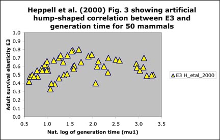
Heppell et al. (2000) included the following
Fig. 3 (on left) and stated:
"Surprisingly adult survival elasticity was not significantly correlated
with generation time. A plot of adult survival elasticity vs. generation
time reveals a hump-shaped correlation where populations with very long
generation times have lower adult survival elasticity (Fig. 3)."
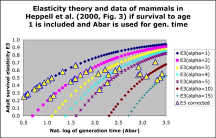
Mollet and Cailliet (2003, Appendix 1.c.i) stated that:
"We suggest that the hump is an artifact of excluding survival to
age one in their elasticity calculation, which leads to an overestimate
of adult survival, in particular for the alpha (α) = 1 and 2 yr species.
If survival to age one is included and if adult survival elasticity is
graphed against Ā instead of μ1, then the relationship is as
expected and follows our Equation 3 in Appendix 1.b with GP = 0: E(adult
survival) = (Ā - α)/(Ā + 1). In the graph below on the right, I used α (alpha) as a parameter
between 1 and 15 yr. We were not able to include the corresponding
figure in our publication but it is shown here on the right below for
comparison with Fig. 3 in Heppell et al. 2000. Data points shown that do not fall on a theoretical line have different alpha than the ones chosen for the theoretical lines (e.g. data points with alpha between 5 and 10 yr). True a solid line for the theoretical calculations would have been much better.
Heppell, S. S., Caswell H., and Crowder L. B. (2000). Life histories and elasticity patterns: perturbation analysis for species with minimal demographic data. Ecology 81, 654-665.
Mollet, H. F. and Cailliet G. M. (2003). Reply to comments by Miller et al. (2003) on Mollet and Cailliet (2002): Confronting models with data. Marine and Freshwater Research 54, 739-744.
The comparison of Fig. 3 in Heppell et al. (2000) with the proposed correction in Mollet and Cailliet (2003) may not clearly reflect where the problem really lies. The above concentrates on only one elasticity, namely the elasticity of adult survival. It is more illustrative to look at the E-pattern comprising the elasticities of fertility, juvenile survival, and adult survival. The E-pattern comprising these three elasticities can be graphed as a single data point in the elasticity triangle introduced by Silvertown et al. (1992) for plants and modified by Heppell et al. (2000) for age-structured animals. If survival to age one is excluded, then the alpha (α) = 1 yr animals are located on the left side of the E-triangle (see below graph on left, which assumes a pre-breeding census as was used by Heppell et al. 2000). If survival to age one is included, then these alpha (α) = 1 yr animals are located on the line which bisects the triangle (see below graph on right). The easiest way to understand that the correct E-patterns must be the one on the right, is to ask where hypothetical animals with alpha (α) < 1 yr would be located in the triangle on the left if they have litters every year and thus require a projection interval (PI) of 1 yr. The correct E-triangle on the right is half-empty and provides the space required for animals with alpha (α) <1 yr and annual reproduction. Note: The difference between the two graphs below is that they used E(F) and called it E(fertility) when in fact E(F) is E(discounted fertility). I suggest they should have used E(m) instead and not mix upper-level E(F) and lower-level elasticities E(Sj) and E(Sa). Then they would have obtained the correct E-triangle as shown on the right.


C) Fig.3 in Mollet (2005, manuscript) used 4 hypothetical species with α = 1, 2, 5, and 15 yr to demonstrate clearly that survival in the discounted fertilities needs to be included when calculating the E-pattern.
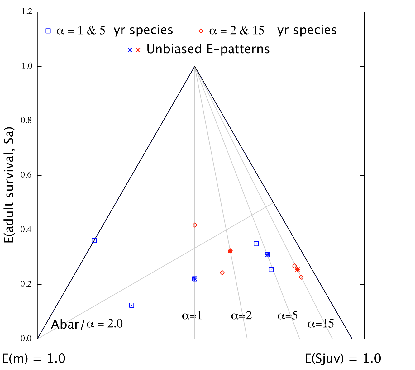
The graph shows four E-patterns for each hypothetical species used (α = 1, 2, 5, and 15 yr). Unbiased E-patterns fall on the corresponding alpha (α) contour and post- and pre-breeding E-patterns coincide. Biased E-pattern for a pre-breeding census (when survival in the discounted fertilities is excluded) fall on the α - 1 contour. Biased E-pattern for a post-breeding census (when survival in the discounted fertilities is excluded) fall between the α and α -1 contours. As alpha (α) increases the bias decreases and the two biased E-patterns approach the unbiased E-pattern. Only one Ā/α contour with value 2.0 is shown.
Note one important conclusion from the above figure. The Ā/α = 2 contour is shown and I proved that E3/E2 = Ā/α - 1. A species located above this contour has E3 largest, a species located below this line has E2 largest. Now consider the α = 2 yr example (first set of red data points on the left). The correct E-pattern for this hypothetical species (vital rates given in Table 1 of manuscript to be added asap) indicates that E2 is largest. However, if a pre-breeding census is used and if first year survival in the discounted fertilities (F = mS1) is not included, then the E-pattern predicts that E3 is largest. If a post-breeding census is used and if adult survival in the discounted fertilities (F = m Sa) is not included, then the E-pattern predicts that E2 is largest. Clearly, pre-breeding and post-breeding census Leslie matrices should produce the same E-patterns. The species in question has no clue about our census model and can have only one E-pattern and it should agree with the one when we use a LHT. I have used the alpha (α) = 2 yr example rather than alpha (α) = 1 yr example where the discrepancies between the different E-patterns are even larger. The alpha (α) = 1 yr example (set of blue data points on the far left) is more complicated and extreme in the sense that if first year survival is not included when calculating the E-pattern using a pre-breeding census, it appears as if an alpha (α) = 1 yr species has no elasticity for juvenile survival. The figure above shows that this incorrect E-pattern is located on the left side of the E-triangle where E(Sj) = 0 [E(Sj) will reach 1.0 at the opposite corner as indicated in Fig. 3 above]. This agrees exactly with the incorrect E-triangle used in Heppell et al. (2000, Fig.1, shown earlier).
D) Fig. 1 in Mollet (2005, rejected, pdf)
E3/E2 = (1/y) {[x/(1 - x)] – [(5y + 1)x(5y + 1)/(1-x(5y + 1))]}. The E3/E2 = 1 contour gives the parameter values of ω/α, Sa/λ, and α for which elasticity of adult survival is the same as elasticity of juvenile survival.
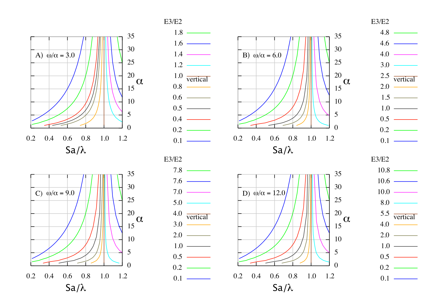
While the above is fairly complicated, it predicts the E3/E2 ratio for all age-structured species with 3 ≤ ω/α ≤ 12 from the vital rates under the usual assumption that m and Sa are age-independent. I suggest that this an important and new result. There is one crucial feature that provides an easy application for elasmobranch. In Fig.1A with ω/α = 3, the vertical contour for E3/E2 is located at Sa/λ = 1. Therefore in the region of most interest, namely Sa/λ < 1, E3/E2 < 1.0. Because most elasmobranchs have ω/α ≤ 3, it follows that for most elasmobranchs the elasticity of juvenile survival [E(Sj)] must be largest without further consideration. For the few elasmobranch with ω/α > 3, Sa/λ is sufficiently smaller than 1 so that they also have E (Sj) largest. In short all elasmobranchs have E3/E2 <1.0. With regard to the elasticity pattern of elasmobranchs it is ω/α which is most important. Age validation is not crucial with respect to the E-pattern because it does not change the ω/α-ratio.
E) What if Sa and m are age-dependent? Covered in Table 3 of Mollet (2005, unpublished)
F)
Fig. 4 in Mollet (2005, unpublished).
Triangle elasticity patterns of elasmobranchs, turtles, mammals, and birds.
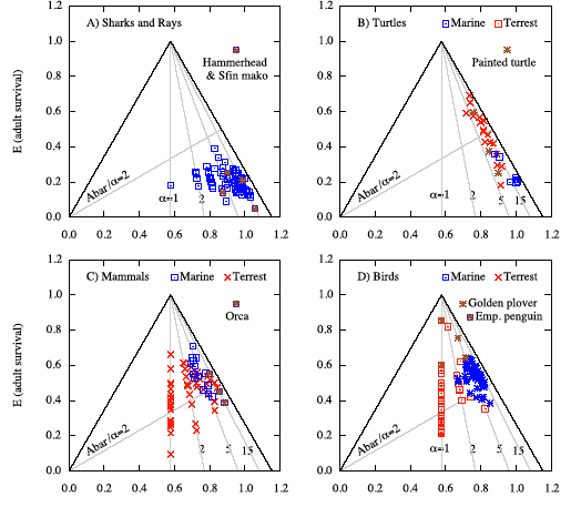 |
Fig. 4 in Mollet
(2005, unpublished).
Triangle elasticity patterns for elasmobranchs, turtles, mammal, and
birds. Contours drawn are for Ā/α = 2.0 and α = 1, 2, 5, and
15 yr. Duplicate star symbols were used for demonstration species: A) Scalloped hammerhead (Hammerhead) with α = 4 and 15 yr (Cortés 2002) and shortfin mako (Sfin mako) with α = 7 yr (Pratt and Casey, 1983) and 18 yr (Natanson et al. in review); B) Painted turtle with 3 sets of different vital rates for 2 populations from Wilbur (1995), Tinkle et al. (1981), and Mitchell (1988); C) Killer whale with 3 sets of different vital rates from Heppell et al. (2000), Eberhardt (2002) and Caswell (2001); D) Golden plover α = 1 yr, ω = 6 & 100 yr, emperor penguin α = 5 yr, ω = 30 & 100 yr (D). Note. E(adult survival) is easiest to understand and is identical with the y-axis. E(fertility) is zero on the left side of the equilateral triangle and reaches 1.0 at the opposite corner located on the bottom side (~1.15, 0). E(juvenile survival) is zero on the right side of the equilateral triangle and reaches 1.0 at the opposite corner on the bottom side (0.0, 0.0 of coordinate system shown). |
Discussion Fig. 4 (Mollet 2005, unpublished, for more see the manuscript)
Fig. 4A for sharks and rays shows that the E-patterns of all elasmobranchs fall below the Ā/α = 2 contour and thus must have E2 > E3. It was already discussed that this must be so on theoretical grounds because ω/α ≤ 3 for most elasmobranchs.
Fig. 4D for marine and terrestrial birds shows that there are several bird species, in particular alpha (α) = 1 yr birds that have E2 > E3 (i.e. elasticity of juvenile survival is larger than elasticity of adult survival. This in conflict with what was claimed by Russell (1999) and Saether and Bakke (2000).
G)
Fig. 1 in Mollet (2004, manuscript).
Comment paper on Oli and Dobson (2003) with title: "Elasticity
Patterns for Mammals: Age at First Reproduction and Mean Age of Reproducing
Females are the Determining Parameters"
There are large differences between the reported elasticities and those calculated here (fig. 1, table 1). The differences are particularly apparent for E(Sj) and E(Sa) of species with population growth rates (λ1) larger than 1.5. For example, for the species with the largest λ1 = 2.619 (Tamias striatus, the eastern chipmunk, α = 1 yr, ω = 7 yr), the reported E-pattern is E(F) ~ 0.70, E(Sj) ~ 0.23, and E(Sa) ~ 0.07. It implies that E(fertility) is about three times as large as E(Sj), which is not possible. The ratio should be one for an alpha (α) = 1 species (see Appendix A10 and A11). The proposed correct E-pattern has E(m) = E(F) = 0.77 (44%), E(Sj) = 0.77 (44%), and E(Sa) = 0.23 (13%).
The discrepancy arises because Oli and Dobson (2003) assumed that the sum of the matrix elements of the E-matrix of an age-structured Leslie matrix is one (e.g. de Kroon et al. (1986); Caswell 2001, p. 230). While technically correct, this overlooks the fact that the discounted fertilities (F) consist of a fertility term (m) and a discount term (Sj and Sa when using a post-breeding census; S1 = survival to age 1 when using a pre-breeding census). The “discount” has to be included when calculating the E-pattern from the E-matrix of a Leslie matrix because otherwise elasticities calculated empirically from a life history table, which only consists of fertilities and survival rates but no discounted fertilities, would not agree with those calculated from the corresponding Leslie matrix. The sum of E(Sj) and E(Sa) alone adds up to 1.0 (Caswell 2001, p. 237; Mollet and Cailliet 2003; see Appendix in this paper for a more general proof). Accordingly, the sum of E(m), E(Sj) and E(Sa) is 1.0 + E(m), rather than 1.0.
In the pre-breeding census the discounted fertilities are F = m S1. If the discount is neglected, it appears as if a species with alpha (α) = 1 yr has zero elasticity to juvenile survival and these species are incorrectly located on the left side of the equilateral elasticity triangle (Heppell et al. 2000, their fig. 1). As alpha (α) increases, the error becomes progressively smaller (see Mollet and Cailliet 2003, Appendix (c) discussing Heppell et al. 2000, their fig. 3). If survival to age one is omitted, the correct E-pattern is easily calculated by adding E(m) to E(Sj), leaving E(Sa) as is, and re-normalizing if desired.
In the post-breeding census used by Oli and Dobson (2003), it is more complicated to correct the E-pattern and it was easier to re-calculate the E-pattern for all 142 species (see 2 Appendix for details). However, there is a further complication when trying to correct the reported E-patterns because Oli and Dobson used a post-breeding census with an ill-advised constant F. In the T. striatus example, this is the source of the difference for E(F) (reported biased 0.70 vs. correct 0.77) because their post-breeding Leslie matrix based on constant F produces a different Ā = 1.42 yr (thus 1/1.42 = 0.70) vs. correct Ā = 1.30 yr based on constant m (thus 1/1.30 = 0.77), although the λ1’s are the same. The λ1’s are the same by design because my m was calculated such that it produced the same λ1. Note that Oli and Dobson (2003) did not calculate Ā and therefore did not realize that their post-breeding Leslie matrix produced a more or less biased Ā for all species but one (Tayassu tajacu, collared peccary, with Sj = Sa).
This is best understood by calculating the fertility schedule that corresponds to a constant-F post-breeding Leslie matrix. For Ochotona princeps (pika or rock rabbit, α = 1, ω = 6 with Sj = 0.111 < Sa = 0.661), it produces an unrealistic fertility schedule with m1 = 0.771/0.111 = 6.95 and m2-m6 = 0.771/0.661 = 1.17. This fertility schedule with m1 much larger than subsequent m’s will lower Ā to 1.50 yr compared to Ā = 2.42 yr for the correctly implemented post-breeding matrix with constant m = 3.28, which agrees with the reported m = 3.25 that did not vary with age (Smith 1974). The majority of mammal populations used by Oli and Dobson (2003) have Sj < Sa, which is as expected, unlike the T. striatus example used previously with Sj = 0.960 > Sa = 0.602 that produced biased Ā = 1.4 > correct Ā = 1.3 yr. The use of a constant-F post-breeding Leslie matrix misrepresents the fertility schedule for the majority of species, including the ones for which age-specific fertilities were reported.
My summary statistics for E(m), (Sj), and E(Sa) of 142 mammals are significantly different (p ≤ 0.003 for re-normalized elasticities) from those reported by Oli and Dobson (2003) which indicates that there is a difference for most species, not just a few outlier species (table 1). Oli and Dobson (2003) reported that the mean absolute value of E(α) = 0.40 was largest, followed by mean E(fertility) = 0.35, whereas I found that mean E(Sa) = 0.54 was largest followed by mean E(Sj) = 0.46, mean E(α) = 0.36, and mean E(m) = 0.32. If the elasticities reported by Oli and Dobson (2003) show large bias, then the results and conclusions of a retrospective elasticity analysis using nested ANOVAs, rank correlation analysis, and nested ANCOVAs with log-transformed body mass as a covariate are of questionable value. The same would apply to a prospective elasticity analysis based on E(m), E(Sj), and E(Sa).
H) On the importance of using actual fertility rather than annualized fertility in the calculation of the E-pattern
The Ā/α ratio (= E(Sa)/E(Sj) + 1 = E3/E2 + 1) perfectly defines the relative importance of adult and juvenile survival and Ā/α = 2 is equivalent to E(Sa) = E(Sj). The relative importance of E(Sj) and E(m) with ratio E(Sj)/E(m) = α needs to be addressed also. When α = 1.0 yr, we have E(Sj) = E(m). For animals with large α, E(Sj) becomes large compared to E(m) and this fact was used in support of management measures that increased juvenile survival because it was far more effective than increasing fertility (e.g. TEDs versus head-start programs for sea turtles (Crouse et al. 1987). However, while E(Sj) is certainly much larger than E(m) when alpha (a) is large, say 15 – 35 yr, the ratio E(Sj)/E(m) would be 3 - 7 instead of 15 - 35, if a projection interval (PI) = 5 yr combined with actual fertility is used instead of PI = 1 yr combined with annualized fertility. Mollet and Cailliet (2003) suggested that this applies to the killer whale and an Australian green turtle population. Many species used in this study have a reproductive cycle (RC) >= 2 yr (e.g. king penguin, several albatrosses, chimpanzee, gorilla, African elephant, hippopotamus, manatee, and several whales). The 66 elasmobranch populations comprise 32 with RC = 1 yr, 29 with RC = 2 yr, and 5 with RC = 2.5(2 or 3) to 3 yr. In all these cases the observed RC combined with actual fertility should be used which will increase the importance of fertility because E(m) becomes larger. In this study I used RC = 1 yr with effective annual fertility for easier comparison with reported results. The E-triangle is suitable for comparison of E-pattern based upon different PI’s. However, it makes identification of a particular species in the E-triangle more difficult because the alpha (a) contours now have units of the PI which will be different for different species, rather than 1 yr for all.
I) Refutation of major comments by reviewers. Actually covered in Mollet (2005, REJECTED, pdf) because I was prepared for everything from the earlier comment manuscript (Mollet, 2004, REJECTED, pdf).
From MF05068Ref1AU.pdf: "It is claimed that there are “conflicting statements” regarding the sum of the elasticities; that is certainly not the case. It is well established that sum of elasticity of population growth rate to matrix entries is always 1.0, and that to life table parameters is 1 + e(m)."
First, it is not well established that elasticities of a life table add up to 1 + e(m). Often (e.g. Cortés 2002) a life history table (LHT) is used to calculate the E-pattern and then the E-pattern is "doctored" so that the sum of the E-pattern is 1.0. This is entirely different compared to calculating the E-pattern correctly and then normalizing it so it can be graphed in the E-triangle.
Second, if the E-pattern of a Leslie matrix or stage-based model is calculated empirically, then the E-pattern will add up to 1 + e(m) not 1.0
Third, my manuscript also showed that when an elasticity pattern of a Leslie matrix is calculated, then the survival rates in the discounted fertilities have to be included such that "elasticity of population growth rate to matrix entries" add up to 1 + e(m) rather than 1.0. The Leslie matrix elements were calculated from the LHT parameters and it makes no sense whatsoever that the sum of the elasticities (the E-pattern) of the vital rates (i.e. fertility, juvenile and adult survival) should be different from that based on a LHT.
From MF05068Ref2AU.doc: "This was an interesting paper, but I think it needs considerable revision before publication. The author makes the appropriate point that biologists need to think carefully about the models that they are using to assess population dynamics in his discussion of the discounted fertilities; however I do not feel that this point is expressed correctly. I would disagree with the author about what he perceives as contradictions between the elasticity matrix and the elasticity patterns."
See again points 1-3 above.
From MF05068Ref1AU.pdf: At a first glance, I thought author’s claim that elasticity patterns are completely determined by α (alpha) and Ā (Abar) was interesting. But looking at eq. A2.4, it is clear that calculation of Ā requires lambda and several life history parameters. So, to say that elasticities can be calculated with alpha and A-bar is the same as saying elasticities can be calculated from all life history variables because all of these variables are needed to calculate lambda.
First, the reviewer missed the point entirely. Alpha (age at first reproduction) and Ā (mean age of the reproducing female at the stable age distribution) are well defined quantities. The formulation of the E-pattern using alpha (α) and Ā is much simpler compared to using lambda and all other life history parameters. The interpretation of the E-patterns also becomes much easier because alpha (age at first reproduction) and Ā (mean age of the reproducing female at the stable age distribution) are well defined quantities and are easier to understand compared to lambda and all other life history parameters (i.e. fertility and survival rates).
Second, I explained why the formulation of the E-pattern in terms of Ā is not included in Caswell (2001) and it is simply due to the fact that Ā is not well-defined for plants which have more complex reproductive cycles compared to age-structured animals.
Third, I'm providing a new closed formula for Ā that is extremely useful for a more theoretical interpretation of E-patterns which was used to calculate the relative proportional importance of adult and juvenile survival for any age-structured animal as a function of Sa/λ and alpha (α) with ω/α treated as an additional parameter. It is true that the closed formula for Ā is only correct if fertility and adult survival rate are assumed to be constant. However, it does not seem to a serious limitation which is demonstrated in paragraph 4.3 of the discussion.
There is really no need to discuss all the anonymous reviewers' comments. They are both wrong on the main point and this led to the rejection of the manuscript. The manuscript could have been shortened considerably once it was accepted and establish that the current theory on E-pattern of age-structured animals is not correct and therefore a summary of the detailed calculation to prove it was and still is badly needed. For example, take Figures 1 and 4 in Heppell, S. S., Caswell H., and Crowder L. B. (2000) which are just plain wrong as outlined in detail in the manuscript and above.